4.7 Applied Optimization
Optimization plays a crucial role in a wide range of disciplines, including the physical sciences, economics, and biology. For example, scientists have studied at what speeds migrating fish swim against a current. In their article "Optimal Swimming Speed in Head Currents and Effects on Distance Movement of Winter-Migrating Fish"(https://journals.plos.org/plosone/article?id=10.1371/journal.pone.0002156), the authors Dr. Jakob Brodersen (et al) write "We conclude that fish are able to adjust both swimming speed and timing of swimming activity during migration to changes in head current velocity in order to minimize energy use."
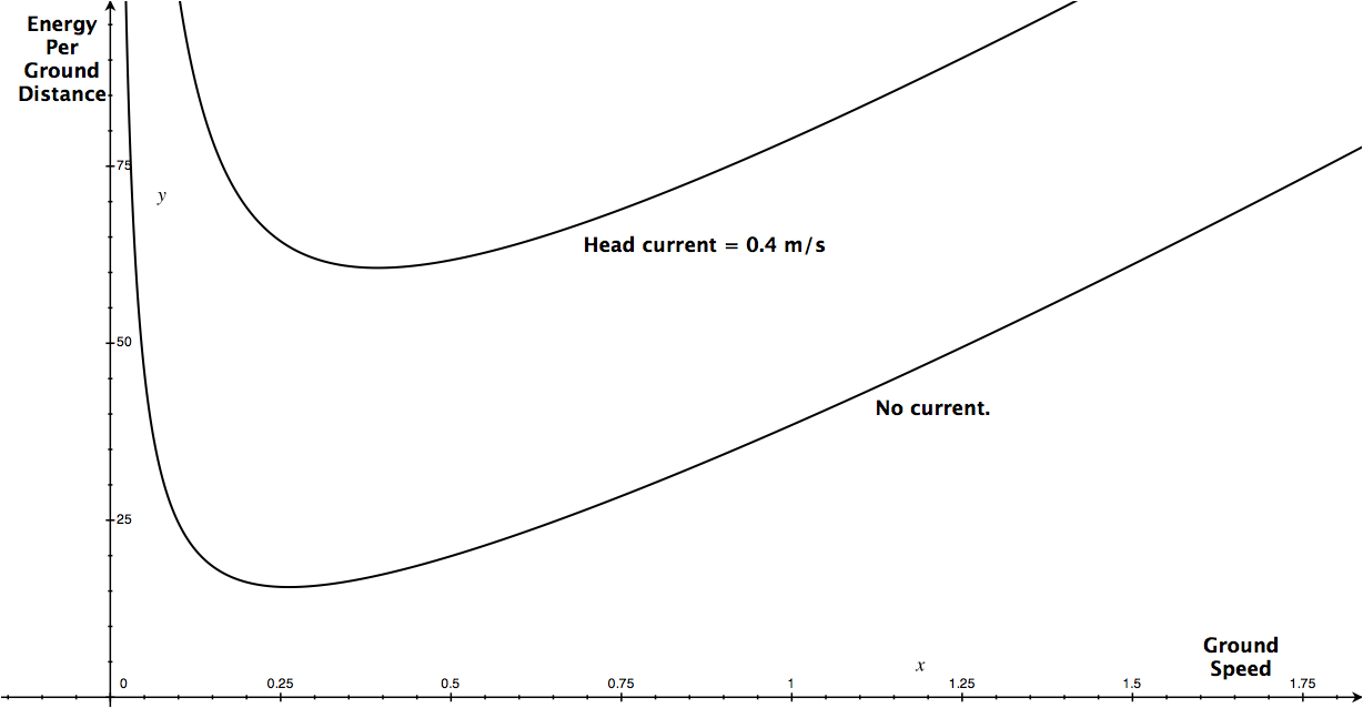
In the figure below, you can see two instances of the relationship between Energy use per ground distance as a function of ground speed at different head currents. In the first case, there is no current, and in the second case the fish swim against a current of \(0.4\text{ m/sec}\). The most energy efficient speed is at the minimal points of the curves, and interestingly, the optimal ground speed varies with the speed of the current. The authors are using a power function model for their calculations but claim to have corroborated their model's predictions through experiments in the field.
We make no claim as to whether the authors of this paper have the correct model since we are not biologists. It should not be a surprise that minimizing your energy expenditure per distance travelled gives a competitive advantage to the fish in a hostile environment, and even that the fish have "figured out" what the optimal speed is can be explained as a consequence of natural selection. But what is of interest to us is that one can use Calculus to investigate the behaviour of fish mathematically, and that we can calculate this optimal speed using our methods.
In many optimization problems, the first step is to write down the objective function. This is the function whose minimum or maximum we need. Once we find the objective function, we can apply the techniques developed in this chapter. Our first examples require optimization on a closed interval \([a, b]\). Let’s recall the steps for finding extrema developed in Section 4.6:
(i) Find the critical points of \(f(x)\) in \([a, b]\).
(ii) Evaluate \(f(x)\) at the critical points and the endpoints \(a\) and \(b\).
(iii) The largest and smallest values are the extreme values of \(f(x)\) on \([a, b]\).
Example 1
A piece of wire of length \(L\) is bent into the shape of a rectangle (Figure 4.68). Which dimensions produce the rectangle of maximum area?

An equation relating two or more variables in an optimization problem is called a “constraint equation.” In Example 1, the constraint equation is
\[ 2x + 2y = L \]
Solution The rectangle has area \(A = xy\), where \(x\) and \(y\) are the lengths of the sides. Since \(A\) depends on two variables \(x\) and \(y\), we cannot find the maximum until we eliminate one of the variables. We can do this because the variables are related: The rectangle has perimeter \(L = 2x + 2y\), so \(y=\frac{1}{2}L-x\). This allows us to rewrite the area in terms of \(x\) alone to obtain the objective function
\[ A(x)=x\left(\frac{1}{2}L - x\right)=\frac{1}{2}Lx - x^2 \]
258
On which interval does the optimization take place? The sides of the rectangle are nonnegative, so we require both \(x \geq 0\) and \(\frac{1}{2}L-x\geq 0\). Thus, \(0\leq x\leq\frac{1}{2}L\). Our problem is to maximize \(A(x)\) on the closed interval \([0,\frac{1}{2}L]\)>.
We solve \(A'(x)=\frac{1}{2}L-2x=0\) to obtain the critical point \(x=\frac{1}{4}L\) and compare:
\begin{align*} \text{Endpoints:}&&A(0)&=0\\ &&A\left(\frac{1}{2}L\right)&= \frac{1}{2}L\left(\frac{1}{2}L-\frac{1}{2}L\right)=0\\ \text{Critical Point:}&&A\left(\frac{1}{4}L\right)&= \left(\frac{1}{4}L\right)\left(\frac{1}{2}L - \frac{1}{4}L\right)= \frac{1}{16}L^2 \end{align*}
The largest value occurs for \(x=\frac{1}{4}L\), and in this case, \(y=\frac{1}{2}L - \frac{1}{4}L = \frac{1}{4}L\). The rectangle of maximum area is the square of sides \(x=y=\frac{1}{4}L\).
Question 4.22 Applied Optimization Progress Check 1
Assume you have 12 yards of fencing material available What is the largest area, measured in square yards, of a rectangular enclosure that has a fenced center divider (so that the final enclosure looks like a domino from above)?
Example 2 Minimizing Travel Time
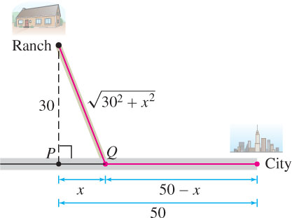
Your task is to build a road joining a ranch to a highway that enables drivers to reach the city in the shortest time (Figure 4.69). How should this be done if the speed limit is \(60\text{ km/h}\) on the road and \(110\text{ km/h}\) on the highway? The perpendicular distance from the ranch to the highway is \(30\text{ km}\), and the city is \(50\text{ km}\) down the highway.
Solution This problem is more complicated than the previous one, so we’ll analyze it in three steps. You can follow these steps to solve other optimization problems.
Step 1. Choose variables.
We need to determine the point \(Q\) where the road will join the highway. So let \(x\) be the distance from \(Q\) to the point \(P\) where the perpendicular joins the highway.
Step 2. Find the objective function and the interval.
Our objective function is the time \(T(x)\) of the trip as a function of \(x\). To find a formula for \(T(x)\), recall that distance traveled at constant velocity \(v\) is \(d = vt\), and the time required to travel a distance \(d\) is \(t = d/v\). The road has length \(\sqrt{30^2+x^2}\) by the Pythagorean Theorem, so at velocity \(v = 60\text{ km/h}\) it takes
\[ \frac{\sqrt{30^2+x^2}}{60}\text{ hours to travel from the ranch to }Q. \]
The strip of highway from \(Q\) to the city has length \(50 - x\). At velocity \(v = 110\text{ km/h}\), it takes
\[ \frac{50-x}{110}\text{ hours to travel from \(Q\) to the city} \]
The total number of hours for the trip is
\[ T(x) = \frac{\sqrt{30^2+x^2}}{60} + \frac{50-x}{110} \]
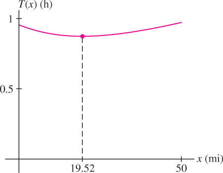
Our interval is \(0 \leq x \leq 50\) because the road joins the highway somewhere between \(P\) and the city. So our task is to minimize \(T(x)\) on \([0, 50]\) (Figure 4.70).
Step 3. Optimize.
Solve for the critical points:
\begin{align*} T'(x)&=\frac{x}{60\sqrt{30^2 + x^2}}-\frac{1}{110} = 0\\[5pt] 110x &=60\sqrt{30^2 + x^2}\implies 11x = 6\sqrt{30^2 + x^2}\\[5pt] \implies 121x^2& = 36(30^2+x^2) \implies 85x^2 =32,400\\[5pt] \implies x&=\sqrt{32,400/85}\approx 19.52 \end{align*}
259
To find the minimum value of \(T(x)\), we compare the values of \(T(x)\) at the critical point and the endpoints of \([0, 50]\):
\[T(0)\approx0.95\text{ h},\quad T(19.52)\approx0.87\text{ h},\quad T(50)\approx0.97\text{ h}\]
We conclude that the travel time is minimized if the road joins the highway at a distance \(x \approx 19.52\text{ km}\) along the highway from \(P\).
Example 3 Optimal Price
All units in a 30-unit apartment building are rented out when the monthly rent is set at \(r = \$1000\text{/month}\). A survey reveals that one unit becomes vacant with each \(\$40\) increase in rent. Suppose that each occupied unit costs \(\$120\text{/month}\) in maintenance. Which rent \(r\) maximizes monthly profit?
Solution
Step 1. Choose variables.
Our goal is to maximize the total monthly profit \(P(r)\) as a function of rent \(r\). It will depend on the number \(N(r)\) of units occupied.
Step 2. Find the objective function and the interval.
Since one unit becomes vacant with each $40 increase in rent above \(\$1000\), we find that \(\frac{r - 1000}{40}\) units are vacant when \(r > 1000\). Therefore
\[ N(r) = 30 - \frac{r - 1000}{40} = 55 - \frac{1}{40}r \]
Total monthly profit is equal to the number of occupied units times the profit per unit, which is \(r - 120\) (because each unit costs $120 in maintenance), so
\[ P(r) = N(r)(r-120) = \left(55 - \frac{1}{40}r\right)(r-120) = -6600 + 58r - \frac{1}{40}r^2 \]
Which interval of \(r\)-values should we consider? There is no reason to lower the rent below \(r = 1000\) because all units are already occupied when \(r = 1000\). On the other hand, \(N(r) = 0\) for \(r = 40 \cdot 55 = 2200\). Therefore, zero units are occupied when \(r = 2200\) and it makes sense to take \(1000 \leq r \leq 2200\).
Step 3. Optimize.
Solve for the critical points:
\[ P'(r) = 58 - \frac{1}{20}r = 0\implies r= 1160 \]
and compare values at the critical point and the endpoints:
\[ P(1000) = 26,\!400,\quad P(1160)=27,\!040,\quad P(2200)=0 \]
We conclude that the profit is maximized when the rent is set at \(r = \$ 1160\). In this case, four units are left vacant.
4.7.1 Open Versus Closed Intervals
When we have to optimize over an open interval, there is no guarantee that a min or max exists (unlike the case of closed intervals). However, if a min or max does exist, then it must occur at a critical point (because it is also a local min or max). Often, we can show that a min or max exists by examining \(f(x)\) near the endpoints of the open interval. If \(f(x)\) tends to infinity at the endpoints (as in Figure 4.72), then a minimum occurs at a critical point somewhere in the interval.
260
Example 4
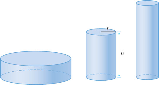
Design a cylindrical can of volume \(900\text{ cm}^{3}\) so that it uses the least amount of metal (Figure 4.71). In other words, minimize the surface area of the can (including its top and bottom).
Solution
Step 1. Choose variables.
We must specify the can’s radius and height. Therefore, let \(r\) be the radius and \(h\) the height. Let \(A\) be the surface area of the can.
Step 2. Find the objective function and the interval.
We compute \(A\) as a function of \(r\) and \(h\):
\[ A = \underbrace{\pi r^2}_{\text{Top}} + \underbrace{\pi r^2}_{\text{Bottom}} + \underbrace{2\pi r h}_{\text{Side}} = 2\pi r^2 + 2\pi rh \]
The can’s volume is \(V = \pi r^{2}h\). Since we require that \(V = 900\text{ cm}^{3}\), we have the constraint equation \(\pi r^{2}h = 900\). Thus \(h = \left(\frac{900}{\pi}\right)r^{-2}\) and
\[ A(r) = 2\pi r^2 + 2\pi r\left(\frac{900}{\pi r^2}\right) = 2\pi r^2 + \frac{1800}{r} \]
The radius \(r\) can take on any positive value, so we minimize \(A(r)\) on \((0, \infty )\).
Step 3. Optimize the function.
Observe that \(A(r)\) tends to infinity as \(r\) approaches the endpoints of \((0, \infty )\):
- \(A(r) \rightarrow \infty\) as \(r \rightarrow \infty\) (because of the \(r^{2}\) term)
- \(A(r) \rightarrow \infty\) as \(r \rightarrow 0\) (because of the \(\frac{1}{r}\) term)
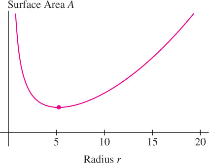
Therefore \(A(r)\) must take on a minimum value at a critical point in \((0, \infty )\) [Figure 4.72]. We solve in the usual way:
\[ \frac{dA}{dr}=4\pi r - \frac{1800}{r^2} = 0 \implies r^3 = \frac{450}{\pi} \implies r= \left(\frac{450}{\pi}\right)^{\frac{1}{3}} \approx5.23\text{ cm} \]
We also need to calculate the height:
\[ h = \frac{900}{\pi r^2} = 2\left(\frac{450}{\pi}\right)r^{-2} = 2\left(\frac{450}{\pi}\right)\left(\frac{450}{\pi}\right)^{-\frac{2}{3}} = 2\left(\frac{450}{\pi}\right)^{\frac{1}{3}} \approx 10.46\text{ cm} \]
Notice that the optimal dimensions satisfy \(h = 2r\). In other words, the optimal can is as tall as it is wide.
261
Example 5 Optimization Problem with No Solution
Is it possible to design a cylinder of volume \(900\text{ cm}^{3}\) with the largest possible surface area?
Solution The answer is no. In the previous example, we showed that a cylinder of volume 900 and radius \(r\) has surface area
\[ A(r) = 2\pi r^2 + \frac{1800}{r} \]
This function has no maximum value because it tends to infinity as \(r \rightarrow 0^+\) or \(r \rightarrow \infty\) (Figure 4.72). This means that a cylinder of fixed volume has a large surface area if it is either very fat and short (\(r\) large) or very tall and skinny (\(r\) small).
The Principle of Least Distance is also called Heron’s Principle after the mathematician Heron of Alexandria (c. 100 AD).
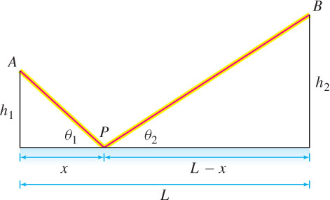
The Principle of Least Distance states that a light beam reflected in a mirror travels along the shortest path. More precisely, a beam traveling from \(A\) to \(B\), as in Figure 4.73, is reflected at the point \(P\) for which the path \(APB\) has minimum length. In the next example, we show that this minimum occurs when the angle of incidence is equal to the angle of reflection, that is, \(\theta _{1} = \theta _{2}\).
Example 6
Show that if \(P\) is the point for which the path \(APB\) in Figure 4.73 has minimal length, then \(\theta _{1} = \theta _{2}\).
Solution By the Pythagorean Theorem, the path \(APB\) has length
\[ f(x) = AP+PB = \sqrt{x^2+h_1^2} + \sqrt{(L-x)^2+h_2^2} \]
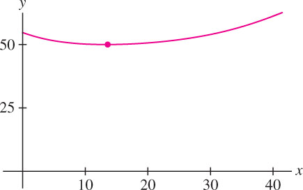
with \(x\), \(h_{1}\), and \(h_{2}\) as in the figure. The function \(f(x)\) tends to infinity as \(x\) approaches \(\pm \infty\) (that is, as \(P\) moves arbitrarily far to the right or left), so \(f(x)\) takes on its minimum value at a critical point \(x\) such that (see Figure 4.74)
\[ f'(x) = \frac{x}{\sqrt{x^2+h_1^2}} - \frac{L-x}{\sqrt{(L-x)^2+h_2^2}}=0\tag{1} \]
It is not necessary to solve for \(x\) because our goal is not to find the critical point, but rather to show that \(\theta _{1} = \theta _{2}\). To do this, we rewrite Eq. (1) as
\[ \underbrace{\frac{x}{\sqrt{x^2+h_1^2}}}_{\cos\theta_1}= \underbrace{\frac{L-x}{\sqrt{(L-x)^2+h_2^2}}}_{\cos\theta_2} \]
Referring to Figure 4.73, we see that this equation says \(\cos \theta_{1} = \cos \theta_{2}\), and since \(\theta_{1}\) and \(\theta_{2}\) lie between \(0\) and \(\pi\), we conclude that \(\theta_{1} = \theta_{2}\) as claimed.
There is also an elegant and simple elementary proof for Heron's principle. For a video of this proof, click here (video to be created).
262
CONCEPTUAL INSIGHT
The examples in this section were selected because they lead to optimization problems where the min or max occurs at a critical point. Often, the critical point represents the best compromise between “competing factors.” In Example 3, we maximized profit by finding the best compromise between raising the rent and keeping the apartment units occupied. In Example 4, our solution minimizes surface area by finding the best compromise between height and width. In daily life, however, we often encounter endpoint rather than critical point solutions. For example, to run 10 meters in minimal time, you should run as fast as you can—the solution is not a critical point but rather an endpoint (your maximum speed).
4.7.2 Section 4.7 Summary
- There are usually three main steps in solving an applied optimization problem:
Step 1. Choose variables.
Determine which quantities are relevant, often by drawing a diagram, and assign appropriate variables.
Step 2. Find the objective function and the interval.
Restate as an optimization problem for a function \(f\) over an interval. If \(f\) depends on more than one variable, use a constraint equation to write \(f\) as a function of just one variable.
Step 3. Optimize the objective function.
- If the interval is open, \(f\) does not necessarily take on a minimum or maximum value. But if it does, these must occur at critical points within the interval. To determine if a min or max exists, analyze the behavior of \(f\) as \(x\) approaches the endpoints of the interval.